
| CapeSym | |
Table of Contents |
SYMMIC can provide compact thermal models for electronic design software to enable electro-thermal co-simulations. In these co-simulations, the operating temperature of a transistor is determined from dissipated power by the compact thermal model. This temperature is used to update the transistor's parameters, usually resulting in a change in the dissipated power. This change feeds back into the compact thermal model which again updates the transistor temperature, and so on. The co-simulation usually settles into a steady-state with stable dissipated powers and temperatures, but electro-thermal simulations can also be used to investigate thermally-induced runaway, such as current collapse in a multifinger HBT.
A compact thermal model is a reduction of the finite element model to an electrical circuit equivalent representation. The resistors in this circuit are thermal resistances (with units Kelvin/Watt) such that dissipated power (W) flows current-like through these resistors to produce a voltage-like temperature change (K) across the resistor. A circuit made up of thermal resistances is sufficient for steady-state simulations, but for transient solutions the compact thermal model must also include thermal capacitances (with units Kelvin/Joule). Therefore, the compact thermal model will be composed of discrete thermal impedances extracted from the continuous physical layers of the finite element model. The calculation of these thermal impedances is the subject of this section.
The compact thermal models provided by SYMMIC are designed to accommodate two types of transistor electrical models, those with temperature parameters and those with thermal ports. For electrical models that do not utilize temperature at all, electro-thermal co-simulation is not possible, but SYMMIC can still be used to evaluate chip temperatures based on the dissipated power calculated by the electronic design software. This process is typically facilitated by a script within the electronic design software that exports the dissipated power for each active device in the layout. The dissipated temperatures are then imported into the layout template using SYMMIC's parameter import facilities.
For transistor models that include either temperature parameters or thermal ports, compact thermal models generated by SYMMIC are sent back to the electronic design software for true electrical-thermal co-simulations. The steps for these co-simulation work flows are briefly outlined here.
Co-Simulation Flow for Temperature Parameters
1. Run steady-state electrical simulation in the Electronic Design Software (EDS).
2. Export device locations and dissipated powers from EDS. This is typically done through a script running within the EDS software environment.
3. The layout is recreated in SYMMIC using device templates that have been configured to represent the thermal stack-up of the MMIC. The dissipated powers are imported into the layout.
4. Run steady-state thermal simulation in SYMMIC to generate either device temperatures (see Run Values section) or thermal resistance equation (see below).
5a. Device temperatures are imported back into the EDS and used to update the temperature parameters of the transistor electrical models. Then go back to Step 1. The whole loop may be automated by EDS script.
5b. The thermal resistance equation generated by SYMMIC is incorporated into the circuit schematic and linked to the temperature parameters and dissipated powers in the electrical circuit. Then iterate the electrical (now electro-thermal) simulation to equilibrium using an EDS script.
Co-Simulation Flow for Thermal Ports
1. Run steady-state electrical simulation in the Electronic Design Software (EDS).
2. Export device locations and dissipated powers from EDS. This is typically done through a script running within the EDS software environment.
3. The layout is recreated in SYMMIC using device templates that have been configured to represent the thermal stack-up of the MMIC. The dissipated powers are imported into the layout.
4. Run steady-state thermal simulation in SYMMIC to generate thermal resistance circuit as netlist (see below). Immediately run transient thermal simulation in SYMMIC, if desired, to add thermal capacitances to the netlist circuit description.
5. Import thermal impedance netlist into the EDS schematic, and attach each port of the thermal network to the thermal port of the corresponding transistor in the layout.
6. Run a complete electro-thermal co-simulation in EDS as either steady-state or transient analysis.
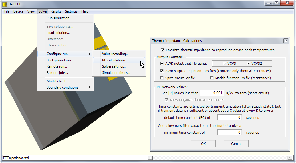
SYMMIC can create a compact thermal model of a layout for a specific set of operating conditions. This calculation is controlled from the Thermal Impedance Calculations dialog, accessed by the Configure run > RC calculations... menu item.
To generate a compact thermal model, the box next to Calculate thermal impedance must be checked. In addition, one or more of the output formats must be selected so that the compact thermal model file(s) will be written at the end of each simulation. The last file that was written can be viewed by selecting Thermal impedance... from the Results menu. A steady-state simulation generates a network of thermal resistances from the peak temperature in each device to the backside boundary condition and to adjacent devices through the common layers. If the steady-state solution is followed immediately by a transient simulation without changing any other parameters, the thermal resistance network will be augmented with thermal capacitances to create a compact thermal model capable of replicating the transient thermal analysis.
Editing, saving or opening the layout will cause any thermal impedance results to be erased from memory. Editing any device parameters in the Device menu will also cause impedance results to be reinitialized. However, parameters configured from the Solve menu can be modified without loss of the results of a prior simulation. This allows a transient simulation to immediately follow a steady-state simulation for computation of dynamic thermal impedance, as described further below.
During the solution, a thermal impedance matrix is created for each of the common layers in the stack-up. The thermal node locations attempt to follow the minimum thermal resistance path from each device maximum temperature spot to the (cold) boundary condition surface. In a bottom-mounted device, for example, the thermal node locations are underneath each device. Conversely, in a top-mounted device, the thermal resistance path may be more circuitous. The thermal impedance matrix for each layer maps the set of dissipated powers in the devices {Pi, i=1..n} to the temperature rises for the devices {DTi, i=1..n} across the layer.
An additional thermal impedance matrix is calculated for the combined topmost layers of the devices. This impedance maps the temperature rise from the top of the common layers to a particular location in each device. This location is usually where the peak temperature occurs. Thus, the compact thermal model allows computation of device peak temperatures from power levels, including thermal coupling between devices.
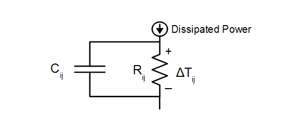
In the simplest form, each thermal impedance component Zij is a thermal resistance. This representation is computed by a steady-state simulation. The AWR scripted equation output format directly implements the matrix multiplications described above. When dynamic impedance information is included, each Zij can be represented by a parallel network of resistance(s) and capacitance(s). This type of representation is output in netlist format as an RC network where power is input as a current and temperature is output as a voltage. The network consists with two separate parts, one for sinking the input currents and another for summing the temperature rises as voltages. Separation of current and voltage pathways is maintained by the use of dependent sources. The thermal RC network can be used in conjunction with transistor models having thermal ports to perform coupled electro-thermal analysis inside the electrical simulator.
To compute the Zij during a simulation, superposition is used to turn on power to one device at a time and measure the resulting temperature rise on each device. Since layouts are normally solved by superposition anyway, the calculation of thermal impedance for a layout does not require any additional effort.
Beginning with version 2.5.5, if the thermal impedances are requested on a device template (not a layout), then SYMMIC first solves the whole model (all device powered), followed by superposition for each flux boundary condition tagged with a unique device number. Device templates created from a layout have this “dn” attribute tag automatically marked on the flux for each active transistor. This is the required approach for solving flip chips. Creating Device Templates from Layouts, in Chapter 4 of the Users Manual, contains a step-by-step procedure for creating a flip-chip ready for thermal impedance calculation.
As noted earlier, the location to which the thermal impedance is calculated is usually where the peak temperature occurs in each device. This is always the case for device templates (even those created using the Export everything option), since the peak locations are known from the initial solution. For a layout, thermal impedance is with respect to the locations in the individual device solutions, whether or not these turn out to be the final peak loci. Initially these locations are placed at the center of each device, but if the superposition calculation is repeated during the solution (as specified by the checkbox in the Solver Settings dialog) then the location is shifted to the device peak. This peak typically occurs in the middle of one of the active fingers of the device, as determined during the part of the calculation with that one device powered. However, in the final combination of the individual device solutions, the actual peak for a device may occur on a different finger due to the influences of adjacent devices. Device locations are set by the first simulation. They remain fixed for subsequent simulations, until the layout is edited, saved or reloaded.
Note: To calculate a separate thermal impedance for each layer in a device template, the layers must have the belongsToMMIC attribute set to “true”. In other words, they must be defined as common layers of the layout, even if no layout is defined.
When a steady-state simulation is followed by a transient simulation with the same constant power levels as used in the steady-state simulation, then the dynamic (transient) impedances are also calculated.
![]()
Rij is the steady-state thermal resistance and tij is the time constant of that thermal resistance rise from zero. Essentially, each thermal impedance represents a parallel RC circuit element through which the power (current) is passed to generate the temperature rise (voltage), such that tij = Rij Cij .
To improve accuracy for impedances of thicker layers, an attempt is made to fit each Zij(t) by two time constants instead of one.
![]()
where Rij = Ra +Rb. The nonlinear regression used to find the parameters of this dual exponential requires at least three time points of Zij(t) to be between 5% and 95% of the steady-state Rij value. If available, more time points in this range will be used to provide a better fit. In contrast, a single time constant can be fit with just one time point in the 5% to 95% range. If no time point is available within the 5% to 95% rise time of Zij, the Rij response is assumed to be instantaneous.
Important note: The transient simulation must provide sufficient data to accurately infer all of the time constants in the solution. Only time points written out in the solution file are used, so the Simulation Times table needs to be configured to output the solution at frequent small time intervals during the fast part of the response. The total simulation time must be sufficient to cover the temperature rise in the slowest device layers and slowest interactions between devices. A reasonable starting point would be the Simulation Times table given below, which can be copied from the example template using Import values from > Template and selecting only the Run Setttings for import.
To get the dynamic thermal impedance from the command line, use the -z flag which causes back-to-back steady then transient simulations to be run on the same template.
> xSYMMIC FETimpedance_layout.xml -z
After completion of a transient simulation, thermal impedance may be examined from the Results menu. If the thermal impedance appears to be in error due to unreasonable or missing C values, the transient simulation can be repeated with new time points defined in the Simulation Times table. The steady-state simulation does not need to be repeated prior to running another transient simulation, as long as the only change is to the integration time steps.
Note: If the Thermal impedance item is grayed in the Results menu but impedance output was expected, make sure that a steady-state simulation was done immediately prior to running the transient simulation. The steady-state resistance calculations have to already be in memory to compute the time constants during the transient. If a transient is run without first running steady-state, all R values in the .bas file will be zero.
The steady-state thermal resistance output is in the form of a Matlab/Octave function (.m file) or a BASIC script (.bas file) that can be imported as a scripted equation into AWR's Microwave Office. Given the array of dissipated powers and the ambient temperature as input, this function returns the array of peak device temperatures. The script can be imported into Microwave Office via the Scripting Editor. By renaming the imported module to “Equations” and then saving and reopening the project, the equation T = Temps(P,T0) can be used in the project to generate the array of device temperatures. Each T[i] value can then be used to set the temperature parameter in each device model. By repeatedly using this calculation and analyzing the circuit, an iterative electro-thermal simulation can be performed.
The scripted equation will only provide accurate temperatures for operating conditions near the original ones. Significantly different cold plate temperatures or device power levels will likely require that a new thermal impedance be calculated because of the temperature-dependent properties of most semiconductor materials. The backside boundary condition is assumed to be a constant temperature cold plate. Any temperature rise on the backside due to a small film coefficient, for example, will not be incorporated in the thermal resistance.
The dynamic thermal impedance is output as a netlist subcircuit, in both AWR Netlist (.net) and SPICE (.cir) formats. The netlist defines an RC circuit that implements the compact thermal model. For a layout with N devices, the circuit has N ports. Each port expects the dissipated power as input current and outputs the peak temperature of the device as a voltage at the port. While the netlist can represent either the steady-state or transient response, the scripted equation represents only the steady-state response. For a transient simulation in Microwave Office, the netlist representation must be used, as illustrated with an example in the next section. The scripted equation for this example is also listed at the end of the section.
As noted above, the separation of current and voltage pathways is maintained in the RC network by the use of dependent sources. When outputting AWR netlist format, the voltage-dependent voltage sources can be either VCVS or VCVS2 circuit elements. The VCVS2 type should be chosen for AWR Design Environment version 10 or higher, as these elements produce the most efficient simulations.
Thermal impedance output was obtained for the generic FET template. A 6-gate full device was centered in a 1x1mm layout. But only half the layout (divided along the midline between the central gates) needed to be simulated, since each half of the solution would be identical. Steady-state for the half-layout was solved with the Repeat superposition box checked, which set the impedance location to the locus of the peak temperature in the device, as described above. The steady-state simulation reported a peak temperature of 422.325 kelvin.
The thermal impedance calculations resulted in two output files representing different forms of the compact thermal model extracted from the steady-state solution. These output files, a netlist circuit description and an AWR scripted equation, are shown below.
! AWR netlist for RC-circuit equivalent thermal ! impedance generated for device power levels: ! Device 0: 0.3 W at (482.25,500,671.025) DIM RES OH ! Rth in K/W CAP F ! Cth in J/K CKT GND 0 CCCS 1 2 0 3 R1=0.001 R2=0 VCVS2 3 6 2 7 R1=190.098 R2=0 VCVS2 6 10 7 11 R1=36.0243 R2=0 VCVS2 10 14 11 15 R1=128.467 R2=0 VCVS2 14 18 15 19 R1=9.99098 R2=0 VCVS2 18 22 19 23 R1=13.4988 R2=0 VCVS2 22 26 23 27 R1=29.6975 R2=0 SHORT 26 30 SHORT 27 31 GND 30 ! sink of power DCVS 31 0 V=T0 ! baseplate temperature DEF1p 1 Rth_network T0=300 |
' AWRDE scripted equation takes an array of dissipated powers P and a backside ' temperature T0 as input and returns array of peak temperatures on the devices Sub Main ' Add function below to (or import this module as) project's Equations script End Sub ' This function generated for T0=300 and device power levels: ' Device 0: 0.3 W at (482.25,500,671.025) Function Temps( P As Double, T0 As Double ) As Double Dim d As Integer, k As Integer, N As Integer Dim T As Double T = T0 ' Half FET Layout layer00 thermal resistance: T = T + 29.6975*P ' Half FET Layout layer01 thermal resistance: T = T + 13.4988*P ' Half FET Layout layer02 thermal resistance: T = T + 9.99098*P ' Half FET Layout layer03 thermal resistance: T = T + 128.453*P ' Half FET Layout layer3b thermal resistance: T = T + 36.0055*P ' Device layer(s) thermal resistance: T = T + 190.103*P Debug.Print "Peak temps due to input power P:" Debug.Print "Device 1: ";T Temps = T End Function |
The AWR scripted equation file (shown above) contains a functional representation of the thermal resistances calculated during the steady-state simulation. Note that the sum of the resistances times the total power of 0.3 W yields the same rise to the peak temperature as produced by the simulation. This can be verified by importing the scripted equation into a Microwave Office project through the Scripting Editor as a project's “Equations” module; then adding an equation to a schematic to report the script's computations:
Next a transient simulation was performed with constant ON power, using the following Simulation Times.
|
Step size (seconds) |
# steps |
t= (seconds) |
|
1.00E-010 |
10 |
1.00E-009 |
|
2.00E-010 |
10 |
3.00E-009 |
|
4.00E-010 |
5 |
5.00E-009 |
|
5.00E-010 |
10 |
1.00E-008 |
|
1.00E-009 |
10 |
2.00E-008 |
|
2.00E-009 |
5 |
3.00E-008 |
|
4.00E-009 |
5 |
5.00E-008 |
|
5.00E-009 |
10 |
1.00E-007 |
|
1.00E-008 |
10 |
2.00E-007 |
|
2.00E-008 |
5 |
3.00E-007 |
|
4.00E-008 |
5 |
5.00E-007 |
|
5.00E-008 |
10 |
1.00E-006 |
|
1.00E-007 |
10 |
2.00E-006 |
|
2.00E-007 |
5 |
3.00E-006 |
|
4.00E-007 |
5 |
5.00E-006 |
|
5.00E-007 |
10 |
1.00E-005 |
|
1.00E-006 |
10 |
2.00E-005 |
|
2.00E-006 |
5 |
3.00E-005 |
|
2.00E-006 |
5 |
4.00E-005 |
|
2.00E-006 |
5 |
5.00E-005 |
|
2.00E-006 |
5 |
6.00E-005 |
|
2.00E-006 |
5 |
7.00E-005 |
|
2.00E-006 |
5 |
8.00E-005 |
|
4.00E-006 |
5 |
1.00E-004 |
|
4.00E-006 |
5 |
1.20E-004 |
|
4.00E-006 |
5 |
1.40E-004 |
|
4.00E-006 |
5 |
1.60E-004 |
|
4.00E-006 |
5 |
1.80E-004 |
|
8.00E-006 |
5 |
2.20E-004 |
|
8.00E-006 |
5 |
2.60E-004 |
|
8.00E-006 |
5 |
3.00E-004 |
|
8.00E-006 |
5 |
3.40E-004 |
|
1.60E-005 |
5 |
4.20E-004 |
|
1.60E-005 |
5 |
5.00E-004 |
|
1.60E-005 |
5 |
5.80E-004 |
|
3.20E-005 |
5 |
7.40E-004 |
|
3.20E-005 |
5 |
9.00E-004 |
|
6.40E-005 |
5 |
1.22E-003 |
|
6.40E-005 |
5 |
1.54E-003 |
|
6.40E-005 |
5 |
1.86E-003 |
|
1.28E-004 |
5 |
2.50E-003 |
|
1.28E-004 |
5 |
3.14E-003 |
|
2.56E-004 |
5 |
4.42E-003 |
|
2.56E-004 |
5 |
5.70E-003 |
|
5.12E-004 |
5 |
8.26E-003 |
|
5.12E-004 |
5 |
1.08E-002 |
|
1.02E-003 |
5 |
1.59E-002 |
|
1.02E-003 |
10 |
2.62E-002 |
|
1.02E-003 |
20 |
4.67E-002 |
This configuration of simulation times provided sufficient resolution during the initial fast response to accurately fit the time constants in the device channel. It also continued the simulation long enough to approach steady-state, ensuring that the long time constants were also adequately represented in the transient. The final peak temperature after 46.7 ms of simulated transient was 420.262 kelvin, 98% of the steady-state value. This simulation took about 40 minutes to run on an Intel Core i7 laptop.
Dynamic thermal impedances were written to the netlist file listed below. Additional resistance values not present in the steady-state result appear because the dual exponential was generated for many Zij to provide a better transient fit. Note that the resistances again add up to a total of 407.7 K/W, corresponding to the correct steady-state temperature rise for the expected power level.
To compare the dynamic response of the compact model to the SYMMIC simulation, the netlist was imported into Microwave Office using Project > Add Netlist > Import Netlist... The subcircuit element created for the netlist was added to a schematic, and a square-wave current source of 300mA (representing 0.3W of dissipated power) was attached to the input port. The Vtime voltage measurement on the port was plotted from the APLAC transient simulator to record the transient response of the circuit. This simulation took just a few seconds in Microwave Office. This plot trace data was exported and compared with the peak temperatures recorded by SYMMIC. The compact model provided a reasonable fit to the transient of the full 3D model, as shown in the following plot of temperature versus log-time.
! AWR netlist for RC-circuit equivalent thermal ! impedance generated for device power levels: ! Device 0: 0.3 W at (482.25,500,671.025) DIM RES OH ! Rth in K/W CAP F ! Cth in J/K CKT GND 0 CCCS 1 2 0 3 R1=0.001 R2=0 VCVS2 3 8 2 9 R1=120.958 R2=0 Cap 3 8 C=3.03975e-11 VCVS2 8 6 9 7 R1=69.1403 R2=0 Cap 8 6 C=1.98253e-09 VCVS2 6 12 7 13 R1=31.1346 R2=0 Cap 6 12 C=8.66253e-09 VCVS2 12 10 13 11 R1=4.89037 R2=0 Cap 12 10 C=2.01458e-05 VCVS2 10 16 11 17 R1=58.8058 R2=0 Cap 10 16 C=6.10626e-08 VCVS2 16 14 17 15 R1=69.6618 R2=0 Cap 16 14 C=1.65275e-06 VCVS2 14 18 15 19 R1=9.99098 R2=0 Cap 14 18 C=2.36215e-05 VCVS2 18 24 19 25 R1=10.9477 R2=0 Cap 18 24 C=4.05756e-05 VCVS2 24 22 25 23 R1=2.55114 R2=0 Cap 24 22 C=0.0131792 VCVS2 22 26 23 27 R1=29.6975 R2=0 Cap 22 26 C=0.00105007 SHORT 26 30 SHORT 27 31 GND 30 ! sink of power DCVS 31 0 V=T0 ! baseplate temperature DEF1p 1 Rth_network T0=300 |
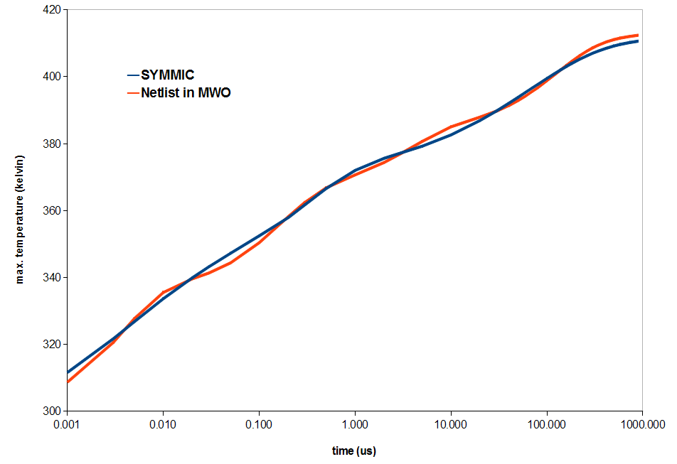
Transient response of
the thermal impedance circuit versus SYMMIC
Although the thermal impedance of the FET was calculated from a layout representation in this example, it may also be calculated from the device representation. This can be done either from the initial device template or from an exported layout. To use the latter approach, use File > Create device template... In the dialog, append nothing and choose to include all components. When the export operation is complete, open the exported device template and adjust the meshing parameters to create a mesh that more closely resembles the original one. Do this by setting Smallest Element Size to 0.25 µm and Largest Element Size to 100 µm. Solving the device for steady-state with this mesh resolution results in a peak temperature of 422.342 kelvin, and thermal resistance values close to those generated for the layout representation. A subsequent transient simulation reproduces the RC thermal network.
The RC calculations... dialog includes a few options for setting limits on values in the RC network. Thermal resistances with absolute values less than 0.001 (K/W) are automatically shorted in the RC network, because such values would have little effect on the device temperatures. The user can increase this minimum R value to eliminate more resistances from the RC network. However, the minimum R has no effect on the scripted equation; all R values are output to the scripted equation no matter how small.
Negative values can occur in the coupling resistances when a device heats another device from below (e.g. through the substrate) while heat spreading cools the device from above. To get the most accurate predictions of temperature, scripted equations and RC networks include these negative thermal resistances when the absolute value is bigger than the minimum R value.
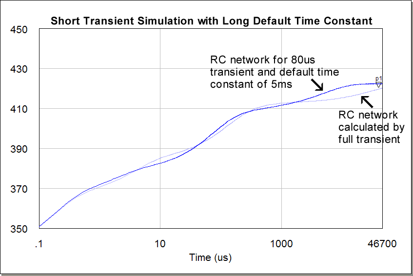
Another option is to set a default time constant for all the thermal resistances in the network. This allows the user to specify a temporal response for the network without running a transient simulation. The default time constant is also applied after a transient analysis to the parts of the thermal network not excited by the transient. Thus, the transient analysis can be run for a relatively short duration to calculate the fastest time constants, and the default value applied to the slower time constants not reached by the simulation. The next figure shows that this approach can sometimes produce a reasonable approximation to calculation of all C values by a long-duration transient simulation.
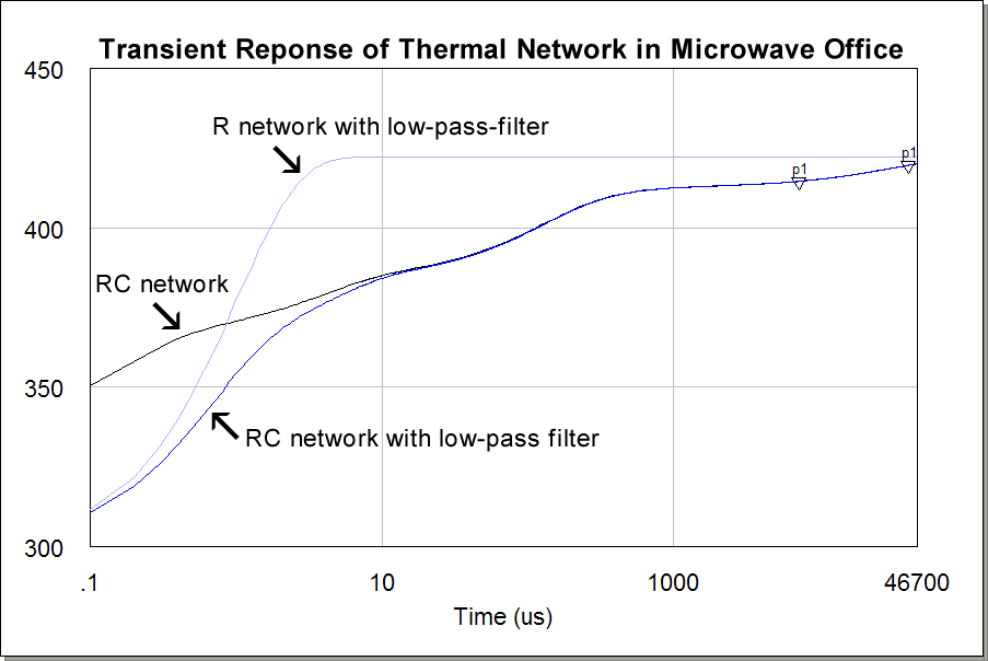
The Thermal Impedance Calculations dialog has an option to add a low-pass filtering thermal capacitor at the input ports to the RC network. This will slow down the response of the thermal network and prevent rapid fluctuations of voltages at the thermal ports. The low-pass filtering option is turned on by typing a non-zero value in the box for the “minimum time constant”. This time constant is divided by the total thermal resistance for each device to generate the value for each filtering capacitor. The low-pass filtering option can be applied to networks generated by both steady-state and transient analysis, as demonstrated in the figure below for the FET example using a time constant of 1 microsecond.
The RC network generated by SYMMIC includes a source that defines the baseplate temperature at the backside of the MMIC. If desired, this source can be made external to the netlist by adding an output port to the netlist and moving the source. Similarly, an output port can be added to allow the attachment of an external resistance to the netlist. This port should be connected to the node sinking all the pathways of the device powers. However, it is important that these two ports not be connected together in any way to avoid duplicating power in the RC network.
For example, an AWR netlist file might end with the following:
:To expose the two additional output ports, the last two lines could be eliminated and the ports modified to:
:This modified netlist could be used in a schematic as shown in the following figure, where a thermal resistance of 84 °C/W (representing a printed circuit board and heat sink) is added to an environmental temperature of 26.85 °C.
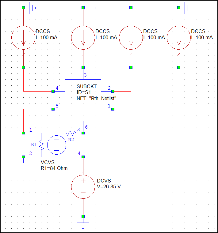
Note that a voltage controlled voltage source is used to maintain the separation of the power (current) and temperature (voltage) pathways. Note also that the accuracy of the resulting thermal network may depend on the temperature-dependent properties of the device materials, since adding the thermal resistance will most likely raise the temperature at which the material properties would be calculated in SYMMIC.
|
<?xml
version="1.0"?> <!DOCTYPE Template SYSTEM "template_format.dtd"> <Template title="Unit cube for which k = L*Q/(dT*A) and Rth = dT/Q"> <!-- L = 1, A = 1, Q = 1 W, dT = 10 K --> <Points> <RefX delta="4/9" refn="4" bias="1.0" /> <RefX delta="1/9" refn="1" bias="1.0" /> <RefX delta="4/9" refn="4" bias="1.0" /> <RefY delta="4/9" refn="4" bias="1.0" /> <RefY delta="1/9" refn="1" bias="1.0" /> <RefY delta="4/9" refn="4" bias="1.0" /> </Points> <ZLayers> <Layer id="layer1" begin="0.0" end="4/9" refn="4" bias="1.0"/> <Layer id="layer2" begin="4/9" end="5/9" refn="1" bias="1.0"/> <Layer id="layer3" begin="5/9" end="1.0" refn="4" bias="1.0"/> </ZLayers> <Materials> <AMaterial id="nice" description="Material with k=0.1" color="226 236 241" conductivity="0.1 300" capacity="1 300" density="1 300" /> </Materials> <Device> <Component name="cube" material="nice" layer="layer1" > <Blocks x="1-3" y="1-3" /> </Component> <Component name="cube" material="nice" layer="layer2" > <Blocks x="1-3" y="1-1" /> <Blocks x="1-1" y="2-2" /> <Blocks x="3-3" y="2-2" /> <Blocks x="1-3" y="3-3" /> </Component> <Component name="center_of_the_cube" material="nice" layer="layer2" record="true" > <Blocks x="2-2" y="2-2" /> </Component> <Component name="cube" material="nice" layer="layer3" > <Blocks x="1-3" y="1-3" /> </Component> </Device> <BoundaryConditions> <Constant temperature="100" face="bottom" layer="layer1" > <Blocks x="1-3" y="1-3" /> </Constant> <SFlux flux="1" face="top" layer="layer3" dn="1" > <Blocks x="1-3" y="1-3" /> </SFlux> </BoundaryConditions> <Simulation> <Time allowUnsteady="true" steady="true" final="25" saveEvery="0.1" step="0.01" > </Time> <Impedance calculate="true" outputBAS="false" outputNET="false" outputCIR="true" /> <Temperature initial="100" useBCfile="false" restartFromFile="false" filetime="0" /> <Record recordAll="false" recordAverageTemps="true" /> </Simulation> </Template> |
The thermal impedance calculations are designed for a layout of one or more devices, but a standalone device template may be modified to generate a compact thermal model under certain conditions. Understanding these conditions will require understanding the device template format as described in the Appendix. The example above models a unit cube (111) with a 1 Watt heat flux on its top surface and the bottom surface fixed at 100 Kelvin.
To compute a thermal impedance, the device must have surface or body flux boundary condition(s) defined on a layer above all of the common layers that have the belongsToMMIC flag set to true. The layer(s) and component(s) on which the flux is defined must NOT have the belongsToMMIC flag. In addition, each flux (or group of fluxes) which will generate a node in the network must be assigned a positive number with the dn attribute, as described in the boundary conditions part of the Appendix.
The thermal conductivity k is set to a nice value so that the temperature rise at the top surface, given by LQ/(kA), is 10 Kelvin. Therefore, the thermal resistance from bottom to top would be 10 Kelvin per Watt. Note, there are no common layers in this device template so that only one "device layer" is generated in the compact model. Also, the SFlux has been given the attribute dn="1" to indicate that it should be included in the compact model.
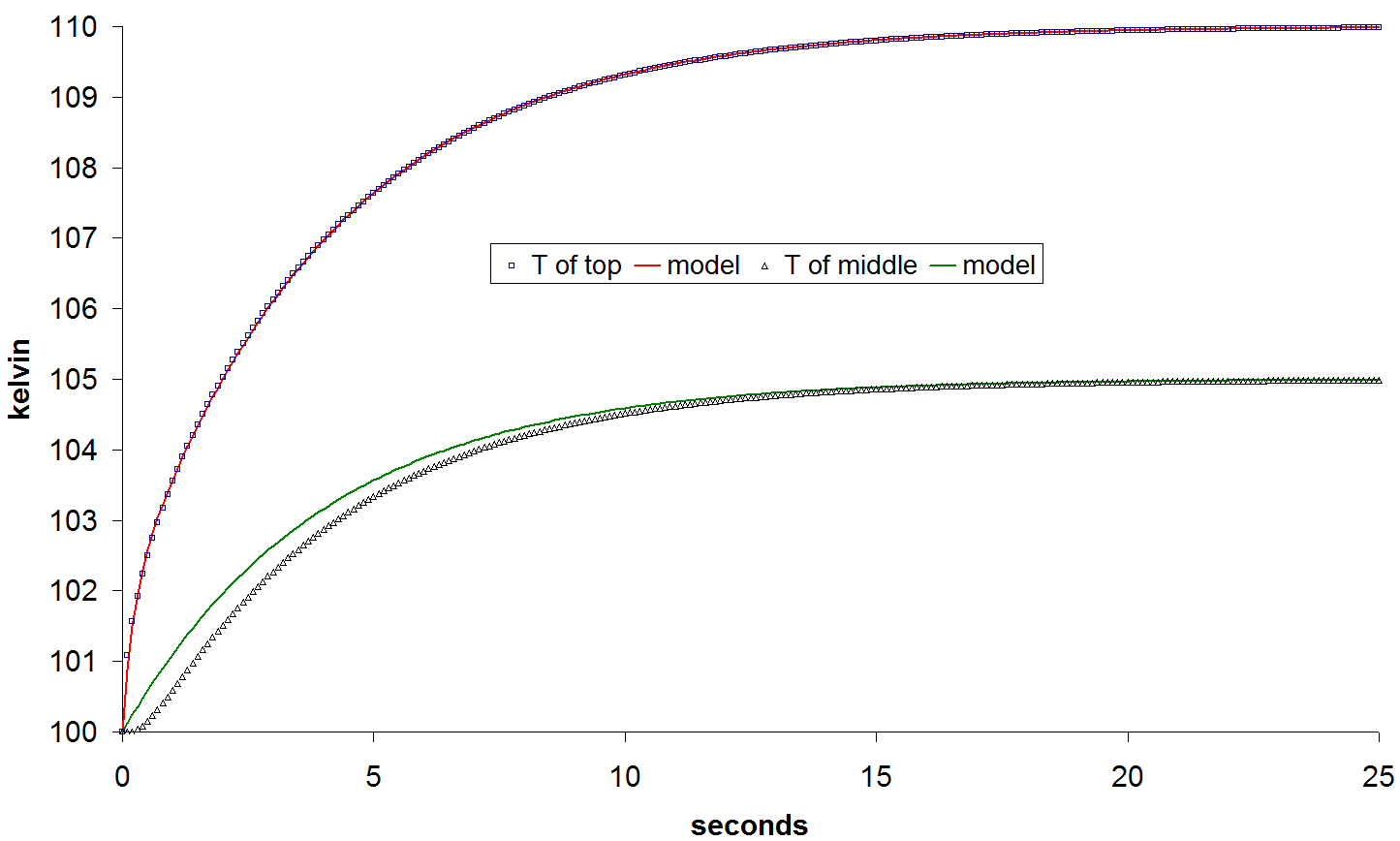
The steady-state solution for this template produces the expected 10 K temperature rise and outputs a spice network with R2=10. To generate the thermal capacitance for the model, the Simulation Times dialog is used to then switch to a Solution through time and the Fill Table button is used to set the time steps, then the simulation is run again. The result is the spice network listed below, where the total Rth=10 has now been divided into two exponential components R2=1.77198 and R3=8.22802, with fast and slow time constants respectively.
* SPICE netlist for RC-circuit equivalent thermal * impedance generated for device power levels: * Device 0: 1 W at (0,0.111111,1) .SUBCKT Rth_network 1 V1 1 2 0 F1 0 3 V1 1 E2 2 9 3 8 1 R2 3 8 1.77198 C2 3 8 0.117009 E3 9 7 8 6 1 R3 8 6 8.22802 C3 8 6 0.486316 R4 6 10 0 R5 7 11 0 R0 10 0 0 V0 11 0 DC 100 .ENDS |
The time constants of the compact thermal model are R2C2 = 0.207 s and R3C3 = 4.00 s. The transient response of the compact model is a good fit to the SYMMIC output, as shown in figure below. The sum of the two exponentials in the model follows closely the maximum temperature at the top of the cube. The rise of the slower component of the model (R3C3) is similar to the rise time of the temperature at the center of the cube, without the delayed onset present in the SYMMIC simulation.
CapeSym > SYMMIC
> Users Manual
> Table of Contents
© Copyright 2007-2024 CapeSym, Inc. | 6 Huron Dr. Suite 1B, Natick, MA 01760, USA | +1 (508) 653-7100