CapeSym

Table of Contents

Temperature Plots

A more detailed picture of the distribution of temperatures in a solution can be obtained from plots generated from the Results menu. Several kinds of plots are available, all of which use the same temperature range, units, and color map used for displaying the 3D temperature distribution. Therefore, the Temperature Scale and its Parameter dialog may be used to adjust the range and colors of any plot.

The temperature probe can be used to assess the approximate temperature on a plot but, unlike a probe on the 3D solution, the probe region for a plot is always a single pixel. The settings in the Probe Spot Size dialog will be ignored when probing any plot.

Please Note: Because plots are rendered in OpenGL, a surface may not be visible from certain viewpoints. For example, when examining a temperature plot of a uniform temperature from front or side views, the perfectly flat surface may not be visible because it is seen edge-on. When examining a temperature plot, rotate the plot slightly to ensure that enough surface is exposed to be visible. Alternatively, display the plot mesh as lines (which have some thickness in any view) by selecting Mesh lines from the Settings menu.

The resolution of temperature plots typically corresponds to the resolution of the finite element mesh in the solution. The default resolution of most device template is usually adequate for creating a smooth plot. But in some cases, such as a plot of a multi-device layout solution, gaps may appear around the edges of devices where the resolution of the mesh in the common areas of the layout is too coarse. The resolution of the common areas is controlled by the Meshsize parameter discussed in the section on Creating and Editing Layouts.

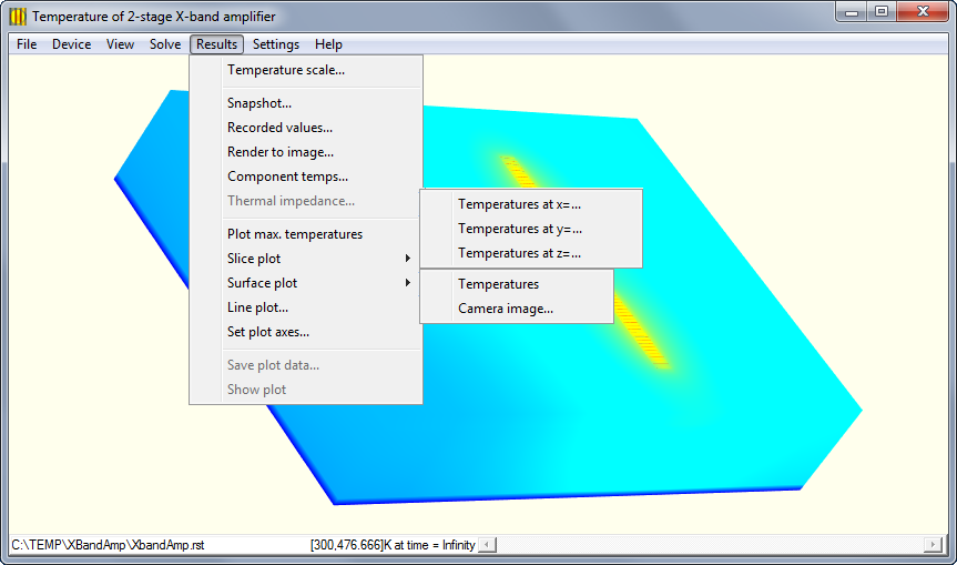
The following figure summarizes the kinds of temperature plots available from the Results menu. In addition to the plot of maximum temperatures and the line plot, there are three types of slice plots and two types of surface plots. Slice plots show the temperatures on an interior plane of the 3D solution. Surface plots show the temperatures on the top surfaces of model visible from the Top view.

Plot of Maximum Temperatures

For the maximum temperature plot, all z values are examined at each (x,y) location in the 3D solution mesh and the maximum temperature value over all these z values is plotted at (x,y). In other words, this plot shows the peak temperatures over the entire device or layout as a 2D surface.

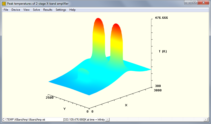
A plot of the maximum temperatures for the X-band amp MMIC.

Slice Plots

The Slice plots show the temperatures at a plane of fracture of the 3D model. The model is sliced at a particular location and the temperatures on the slice face are interpolated from the 3D solution mesh. The slice face is then plotted in 2D with the temperatures at each (x,y) point displayed on the z-axis.

Plot of Temperature at X

This command plots the temperature over all (y,z) points in the solution at a slice plane defined by a user-specified x value. For example, if a device extends from 0 to 272 microns along the x-axis, a plot at x=136 will generate a surface representing the temperature for every (y,z) position on a plane through the center of the device. The (y,z) locations displayed in the plot are located at the nodes of the solution mesh. If the x-plane does not correspond to a plane of mesh points, the temperature is linearly interpolated between the two nearest mesh planes. At (y,z) locations outside of the mesh, no temperature data is plotted.

Plot of Temperature at Y

This command plots the temperature over all (x,z) points in the solution at a slice plane defined by a user-specified y value. For example, if a device extends from 0 to 420 microns in the y-direction, a plot at y=210 will generate a surface representing the temperature for every (x,z) position on a plane through the center of the device. The (x,z) locations displayed in the plot are located at the nodes of the solution mesh. If the y-plane does not correspond to a plane of mesh points, the temperature is linearly interpolated between the two nearest mesh planes. At (x,z) locations outside of the mesh, no temperature data is plotted.

Plot of Temperature at Z

For a z-plane plot, the user enters the z-value for the slice plane as a distance from the bottom surface of the device or layout. For example, if a device extends from 0 to 673 microns in z, a plot at x=336.5 will generate a surface representing the temperature for every (x,y) point on a plane through the center of the device. The (x,y) locations displayed in the plot are located at the nodes of the solution mesh. If the z-plane does not correspond to a plane of mesh points, the temperature is linearly interpolated between the two nearest mesh planes. At (x,y) locations outside of the mesh, no temperature data is plotted.

Surface Plots

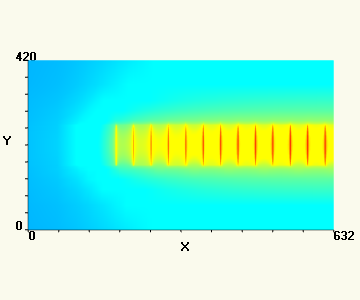
Surface plots show temperatures at the top surface of the model, as might be measured by a thermal camera looking down on the chip. The surface plot of Temperatures shows the actual mesh at the top of the 3D solution, at the full resolution of the solution finite elements. The Camera image... surface plot reinterpolates and averages the actual temperatures to produces an array of rectangular pixels similar to the image produced by the thermal imager. Each pixel has a single temperature value.

The following figure demonstrates the difference between the actual solution temperatures and a camera image generated from them. Note the lower resolution of the image plot which has a significantly lower peak temperature. While the actual temperatures at the surface exhibit a peak of 476.666 K, the hottest pixel in the image plot is only 455.559 K, a difference of more than 30 degrees celsius. The difference is due to the area-weighted averaging that generates pixel temperatures from the solution mesh at the top surface.

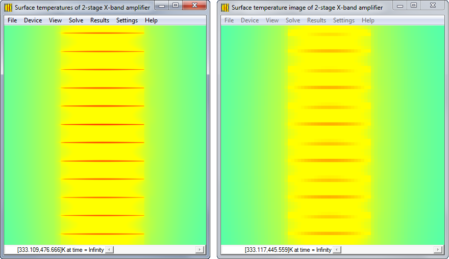
Surface plot of Temperatures (left) versus surface plot of Camera image (right).

The above surface maps were generated for the X-band amplifier MMIC described in an earlier chapter. The Camera image... surface plot on the right side of the figure was generated from the parameters settings in the Surface Image Map dialog shown below. Pixel Size was chosen to be 5 microns, to emulate the expected resolution of a mid-wave infrared (MWIR) camera. To match the actual top surface area of the layout of 3800x2500 microns, the Image Size was set to 760x500 pixels and placed at the origin of the model (0,0).

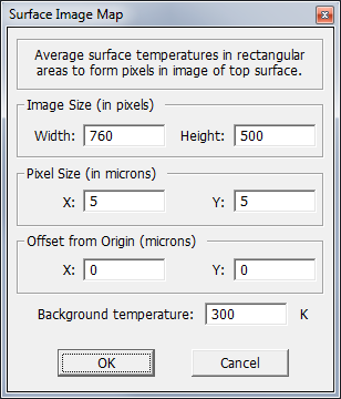
The Surface Image Map dialog includes a parameter for the Background temperature of the thermal imager test setup. Any pixels which lie wholly outside of the model are assigned this temperature. Pixels overlapping the borders of the model, will generate an area-weighted average that is part model temperatures and part background temperature, based on the amount of overlap with each region.

Plot of Temperatures Along a Line

The Line plot... menu item generates a 1D plot of the average temperatures around points along an arbitrary straight line through the solution, as depicted in the following figure. The black outline in the figure depicts the template volume, while the red line is the trajectory of the 1D plot. At each point along the line a volume is used for averaging, represented by the blue cube.

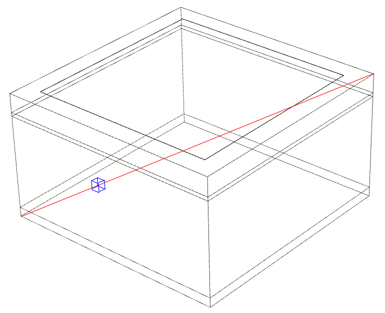
Calculating average temperatures in rectangular boxes along a straight line.

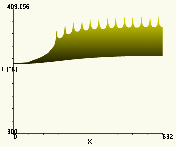
To give a specific example, a line plot is made at the top of the substrate through the second stage of the X-band amplifier example. For this plot the Line Plot dialog is filled as shown.

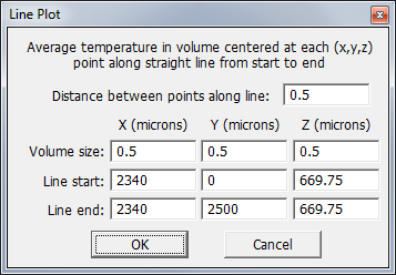
The Line Plot dialog allows the user to enter the starting and ending locations of the straight line, as well as the size of the volume in which to average temperatures at each point. The minimum size for the averaging box is 0.002 microns in any dimension. Values less than this will be reset to the minimum value before extracting the plot. The number of points in the plot is determined by the length of the line and the Distance between points along line: value. In this example, the line passes through the top of the substrate from (2340,0,669.5) to (2340,2500,669.5). Along this distance of 2500 microns, the average temperature will be computed every 0.5 microns, giving a total of 5000 points in the plot. At each point, the temperature is averaged in a volume of 0.5x0.5x0.5 microns centered on the point.

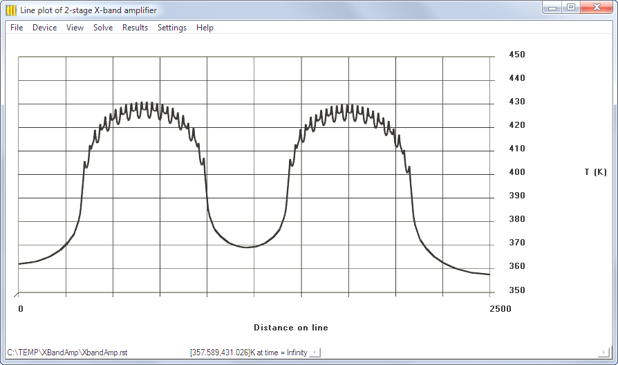
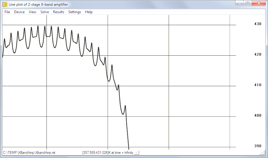
Here, the plot axes were adjusted to display a grid on the XT plane, with T ticks labeled every 10 degrees kelvin. Because the plot is made in the same drawing context used for the rest of the graphical display, adjustment of the plot view utilizes the menu, mouse, and keyboard commands described previously. For example, dragging with the right mouse pressed allows magnification to observe the plot in finer detail.

Plot Axes Dialog

The Plot Axes dialog allows the user to configure the axes of the plot. Unchecking one of the Show labels boxes results in all text being removed from that axis, while unchecking a Show axis box results in the axis and its tick marks being removed from the display. Use Frame to create a 3D box around the plot, and use the Show grid check boxes to create a grid of lines on one plane of the bounding box. The dialog also allows the number of intervals (where tick marks are drawn) to be set on each axis. By default each axis is divided in 10 equal intervals, resulting in 9 tick marks between end points of the axis.

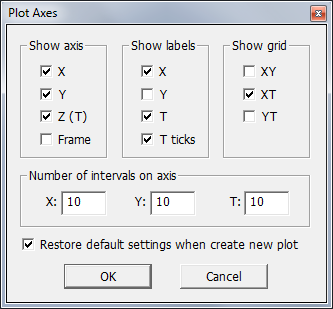
Each plot type has a default axis configration. For example, the line plot displays labels for only the X and T axes by default. The default axis configuration can be changed, but it will be restored when the next plot is generated. Unchecking the box next to Restore default settings when create new plot prevents automatic resotration of the default axis configuration every time a plot is generated. Instead, the user's configuration will remain the same for all plots.

Show Device or Plot

Only one temperature plot can be displayed at a time, but the display can be switched from the plot to the 3D solution by selecting the Show device/layout item at the bottom of the Results menu. The temperature plots are rendered in orthographic mode so that there is no perspective distortion. In contrast, the device template and solution are rendered in perspective mode to give a realistic 3D display.

Save Plot Data

The Results menu includes a command for saving plot data. A plot can be exported to a file in either of two formats: comma separated values format or Tecplot format. These formats are similar to the plain text formats used for saving the 3D solution, but the Tecplots formats are different because the plot data is not 3D. Furthermore, the camera image plot temperatures pertain to areas (pixels) instead of vertices, so the .csv format for this plot is different from the standard format. Likewise, because the line plot is not 2D, there is a different Tecplot format for it.

Standard CSV Format for Plots

The .csv solution file format consists of lines of plain text terminated by newline characters. The file can be read by any text editor or spreadsheet. The first line of the file is the header containing the title of each column separated by commas. This is followed by the data for each time point in the solution. Each data line consists of time, x, y, z, temperature, separated by commas. Each (x,y,z) triplet represents a node of the 2D plot mesh. The nodes are listed in ascending order by z, then by y, then x. That is, the x values ascend most rapidly, restarting at each new y value. Nodes can be re-ordered by sorting rows in a spreadsheet.

The following partial listing demonstrates the format of the standard .csv file:

time,x,y,z,temperature
Inf,  0.000000000E+00,  0.000000000E+00,  0.000000000E+00,  3.620840139E+02
Inf,  1.000000000E+00,  0.000000000E+00,  0.000000000E+00,  3.620920567E+02
Inf,  2.000000000E+00,  0.000000000E+00,  0.000000000E+00,  3.621024127E+02
Inf,  3.000000000E+00,  0.000000000E+00,  0.000000000E+00,  3.621127714E+02
Inf,  4.000000000E+00,  0.000000000E+00,  0.000000000E+00,  3.621231333E+02
 :

Camera Image CSV Format

When a surface plot is generated using the Camera image... command, the resulting plot has meaningful temperatures only for each pixel region, instead for each vertex, so a different format is used to save this type of plot data. The temperature for each pixel is output along with the (x,y) coordinates of the center of the pixel. These coordinates are the location of the pixel on the top surface of the model relative to the origin at (0,0).

The following partial listing demonstrates the format of the camera image .csv file:

time,x,y,temperature
Inf,  2.500000000E+00,  2.500000000E+00,  3.338446551E+02
Inf,  7.500000000E+00,  2.500000000E+00,  3.338583016E+02
Inf,  1.250000000E+01,  2.500000000E+00,  3.338719482E+02
Inf,  1.750000000E+01,  2.500000000E+00,  3.338855947E+02
Inf,  2.250000000E+01,  2.500000000E+00,  3.338992412E+02
 :

Tecplot Format for 2D Plots

The Tecplot data file format consists of lines of ASCII text terminated by newline characters. The file can be read by any text editor. The first line contains the title, the second line contains the variable names, and the third line contains the description of the “zone” of data. Each zone specifies the temperatures over a finite element mesh. The first zone contains the (x,y,z) positions of the mesh nodes and a set of indices describing how these nodes are grouped into finite elements. The third line of the file is the header for the first zone, giving the number of nodes (N) and the number of finite elements (E). The node data begins on the fourth line.

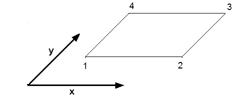
Each of the N node lines is composed of floating point values for the x, y, and z coordinates (in microns) and a temperature value (in kelvin) for a node. The N node lines are followed by E lines containing the element indices. Each element of type FEQUADRILATERAL is a rectangular area with 4 corners at the (x,y,z) node points. Each line specifies the node index (an integer from 1 to N) of each corner in the order shown in the figure.

For solution files with only 1 time point (e.g. steady-state solutions), the file does not contain any additional data. But for solutions through time, the first zone may be followed by any number of additional zones containing node locations and temperature values for subsequent time points. Each zone begins with a header line that repeats the number of nodes N and finite elements E for the mesh. The zone header also includes a SOLUTIONTIME value that gives the time (in seconds) for this zone. The header line is followed by N lines containing the N vertices of the mesh and their temperatures.

The following partial listing demonstrates the format:

TITLE = "Tecplot Output"
VARIABLES  = "X" "Y" "Z" "temperature"
ZONE T="  0.000000000E+00", N=5644, E=4536, ZONETYPE=FEQUADRILATERAL, DATAPACKING=POINT, SOLUTIONTIME=  0.000000000E+00
  0.000000000E+00   0.000000000E+00   3.000000000E+02   3.000000000E+02
  4.098360656E+01   0.000000000E+00   3.000000000E+02   3.000000000E+02
  7.377049180E+01   0.000000000E+00   3.000000000E+02   3.000000000E+02
  1.000000000E+02   0.000000000E+00   3.000000000E+02   3.000000000E+02
  0.000000000E+00   4.098360656E+01   3.000000000E+02   3.000000000E+02
  :
  2.500000000E+02   2.600000000E+02   3.000000000E+02   3.000000000E+02
    1    2    6    5
    2    3    7    6
    3    4    8    7
    4   17   19    8
    5    6   10    9
    :
 5641 5642 5644 5643
ZONE T="  1.000000000E-06", N=5644, E=4536, ZONETYPE=FEQUADRILATERAL, DATAPACKING=POINT, SOLUTIONTIME=  1.000000000E-06,CONNECTIVITYSHAREZONE=1
  0.000000000E+00   0.000000000E+00   3.000000000E+02   3.000000000E+02
  4.098360656E+01   0.000000000E+00   3.000000000E+02   3.000000000E+02
  7.377049180E+01   0.000000000E+00   3.000000000E+02   3.000000000E+02
  1.000000000E+02   0.000000000E+00   3.000000000E+02   3.000000000E+02
  0.000000000E+00   4.098360656E+01   3.000000000E+02   3.000000000E+02
  :
  2.500000000E+02   2.600000000E+02   3.007075130E+02   3.007075130E+02
ZONE T="  2.000000000E-06", N=5644, E=4536, ZONETYPE=FEQUADRILATERAL, DATAPACKING=POINT, SOLUTIONTIME=  2.000000000E-06,CONNECTIVITYSHAREZONE=1
  0.000000000E+00   0.000000000E+00   3.000000000E+02   3.000000000E+02
  4.098360656E+01   0.000000000E+00   3.000000000E+02   3.000000000E+02
  7.377049180E+01   0.000000000E+00   3.000000000E+02   3.000000000E+02
  1.000000000E+02   0.000000000E+00   3.000000000E+02   3.000000000E+02
  0.000000000E+00   4.098360656E+01   3.000000000E+02   3.000000000E+02
  :
  2.500000000E+02   2.600000000E+02   3.016295207E+02   3.016295207E+02
ZONE T="  3.000000000E-06", N=5644, E=4536, ZONETYPE=FEQUADRILATERAL, DATAPACKING=POINT, SOLUTIONTIME= 3.000000000E-06, CONNECTIVITYSHAREZONE=1
  0.000000000E+00   0.000000000E+00   3.000000000E+02   3.000000000E+02
  4.098360656E+01   0.000000000E+00   3.000000000E+02   3.000000000E+02
  7.377049180E+01   0.000000000E+00   3.000000000E+02   3.000000000E+02
  1.000000000E+02   0.000000000E+00   3.000000000E+02   3.000000000E+02
  0.000000000E+00   4.098360656E+01   3.000000000E+02   3.000000000E+02
  :

Tecplot Format for Line Plots

The Tecplot data file format for line plots is 1D instead of 2D, the quadrilateral elements are dispensed with. The first two header lines are the same, but the third line specifies a line of the I number of points. This line is repeated for every time point in the solution. The I lines of data follow, with the X values giving the distance along the line and the Z and temperature values both giving the temperatures.

The following partial listing demonstrates the line plot Tecplot format:

TITLE = "Tecplot Output"
VARIABLES  = "X" "Y" "Z" "temperature"
ZONE T="Inf", I=2501, ZONETYPE=ORDERED, DATAPACKING=POINT
  0.000000000E+00   0.000000000E+00   3.620826798E+02   3.620826798E+02
  1.000000000E+00   0.000000000E+00   3.620919425E+02   3.620919425E+02
  2.000000000E+00   0.000000000E+00   3.621023016E+02   3.621023016E+02
  3.000000000E+00   0.000000000E+00   3.621126620E+02   3.621126620E+02
  4.000000000E+00   0.000000000E+00   3.621230237E+02   3.621230237E+02
  5.000000000E+00   0.000000000E+00   3.621333873E+02   3.621333873E+02
  :