CapeSym

Table of Contents

Solutions Through Time

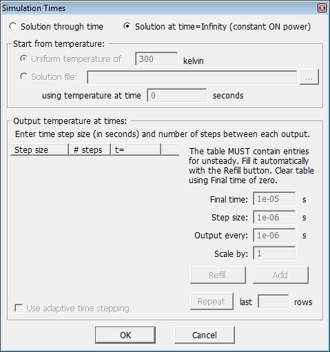
SYMMIC can be used to obtain transient (or unsteady) solutions as well as steady-state solutions. The choice is made in the Simulation Times dialog, depicted in the figures below. The Simulation Times dialog is accessed from the Solve menu by the Simulation times... item in the Configure run submenu.

Checking the circle next to “Solution at time=Infinity” results in only the steady-state solution being computed. All other time and initial condition parameters in the dialog are irrelevant to this solution, so these boxes are grayed. The temperature solution at a particular time (after t=0) can be obtained by selecting “Solution through time” instead. For an unsteady solution to be computed, two additional types of information are required: the initial temperature and the integration time steps.

Solving Unsteady Finite Element Equations

The solution through time involves inverting the system matrix given by (M + Δt K), where Δt is the time increment for the integration step. See the Temperature Computations section for the equation to be solved. The Δt values are the Step size entries in the table in the Simulation Times dialog. This table also groups together the number of steps to be taken between outputs to the solution file. So each row of the table defines a time interval with a number of steps at a specific Δt. The solution is written out at the end of the interval. Each row can use a different Δt, which means that (M+ΔtK) may be changing over each output interval.

The default behavior of the unsteady solver is to analyze, reorder and symbolicly factor (M+ΔtK) on the very first time step in the first interval. Prior to version 2.9.0, all subsequent intervals and time steps made use of the same analysis for numerical factorization and iterative refinement, which is sufficient for solving most problems. Efficiency improvements may be realized by periodically reanalyzing and refactoring (M+ΔtK) as it is changing during the solution. SYMMIC now allows control of when the unsteady solver does a full analysis and refactoring of (M+ΔtK).

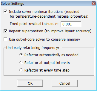
In the Solver Settings dialog (Solve > Configure run > Solver settings...) three choices are available for the Unsteady refactoring frequency. The default behavior is Refactor automatically as needed. In this mode of operation the solver monitors the time to iterate to a solution using the current factorization. If this time exceeds 33% of the time it took for the last full analysis and refactorization, a full analysis and refactorization of (M+ΔtK) is done before the next time step is solved.

The Refactor at output intervals option explicitly analyzes and factors (M+ΔtK) at the start of each output interval (i.e. each row in the table). Refactor at every time step explicitly analyzes and factors (M+ΔtK) for every Δt within every interval. The last option is definitely the slowest, but there is the possibility of improved accuracy if M and K are changing rapidly due to temperature-dependent material properties.

To get an idea of the performance differences between the refactoring frequencies, consider a solution through time for the 13-gate generic FET template using the time steps and intervals given in the Thermal Impedances of a FET section. In this example, Δt is changing with almost every interval. As shown in the table below, the new unsteady solver is at least twice as fast as the prior version, with less than 0.005 ºC differences between the outputs. The fastest simulation is obtained by refactoring every output interval.

Note: Refactoring is only applicable to the default Pardiso solver. It does not apply to any of the iterative solvers, such as the preconditioned conjugate gradient solver, used for running xSYMMIC on clusters.

Start From Temperature

Two options are available for choosing the initial temperature condition: a uniform temperature over the whole device, or a previously computed temperature solution. In the later case, the solution file containing the desired initial state is specified along with the particular time point in that file. This initial condition will become the first temperature in the output file generated when the new simulation is run. However, the time point of the initial condition in the new solution will always be reset to t=0. No matter what restart time is specified, time will be restarted at zero for the new simulation. If the initial condition is a uniform temperature, then the solution will contain that uniform temperature at time t=0. The second time point in the file will be the temperature computed at the end of the first output interval.

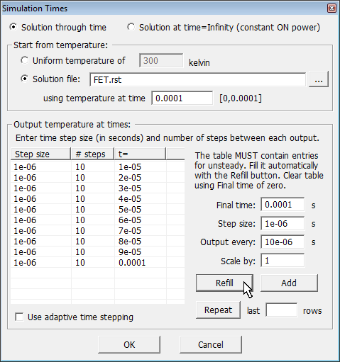
When the restart solution filename is edited or selected using the browse (...) button, the range of times available in the solution file will be updated in the dialog and the last available time point will be automatically filled in as the desired starting point. Edit the time field AFTER selecting the filename to set a time other than the last time in the file. A steady-state solution can be used as the initial temperature by specifying the filename and selecting -1 as the time, since -1 is used to represent t=infinity in the file.

Note: The solution file used for restart must have been generated with the same set of template parameters as the current problem. If the current mesh is not identical to the one in the solution file, the solver will exit with an error message.

Note: Restart from file is not available for a simulation of a layout containing multiple devices. To restart from a file initial condition, the layout would need to be exported to a device template first, so that the restart file can be generated and used on this representation instead.

Output Temperature at Times

All unsteady solutions require that a step size be chosen for temporal integration. This value must be small enough to ensure the accuracy of the numerical solution, and is problem dependent. The user must specify the integration step size and number of steps per output for the unsteady simulation by entering values in the table. When in unsteady mode, the dialog will not respond to the OK button unless the output temperature table contains entries.

In each row enter the integration step size in the first column and the number of steps to complete before recording the temperature in the second column. The third column will then be automatically updated with the total simulations time up to that row. Device temperatures will be output at each time point corresponding to a row of the table. For the example shown in the figure above, a step size of 1µs was chosen. The entire simulation thus involved 100 time steps, with every 10^th step recorded to the solution file. The solution at time t=100µs (0.0001s) will be saved along with solutions at times 10, 20, 30, ..., 90 µs.

To enter data, click on one of the table elements with the mouse to begin editing it. Use the Tab key to move to the next column in the table, or the Enter key to move to the next row. Use the Insert key to stop editing and to insert a new row. Use the Delete key when not editing to delete a row. When editing, use the Insert key to select a row to be deleted.

The table may be filled in automatically by adjusting the parameters to the right and clicking the Refill button. The Refill button clears the table of all entries prior to refilling. So to clear the table of all entries, enter a value of zero for the Final time and then press Refill.

Note: The table may be slow to fill if parameters are used that would create more than 65,535 entries. If too many table rows would be created when filling the table, the user is given the option to cancel the operation before it begins.Note that there may be a limit to the number of rows that the table can handle efficiently, so warnings are provided at 65,535 entries. Longer problems can be simulated by creating a series of device templates using the solution from each previous stage as the initial temperature.

To add rows to the table rather than refilling it, use the Add button. When the Add button is pressed the Final time is interpreted as an increment beyond the current last row of the table, and subsequent rows are filled accordingly. Using the Add button with a Final time of zero does not add any rows to the table, but will remove any blank rows that are present between non-blanks ones.

To create a periodic pattern of time steps, first enter the number of rows at the end of the table that are to be repeated in the last ____ rows edit box, and then press the Repeat button. The specified number of rows will be copied from the end of table and appended to it. The Repeat button can be used any number of times to add rows to the end of the table. When a number of rows greater than the length of the table is specified, the entire table will be duplicated.

Gradually Increasing Integration Steps

For devices with very small heating elements, such as near the narrow gates of a FET, an accurate transient simulation of gate temperatures will require very small integration steps, perhaps in the sub-nanosecond range. For these types of problems it is desireable to use a small time step initially to accurately model gate heating and then gradually increase the step size as the change in gate temperature slows down.

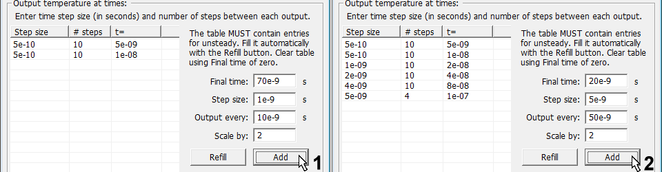
The Scale by edit box was designed to aid in the creation of simulations with increasing integration time steps. When a number greater than 1 is entered, the Add or Refill buttons will increase the step size and output intervals on each row until the final time is reached. For example, setting Scale by to 2 and using a 1µs step size and 10µs output interval, results in doubling of the step size in each row as shown in the following table entries.

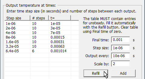
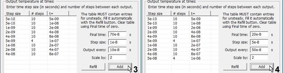
By doubling the step size, a long transient can be more efficiently simulated. For example, a fixed step size of 0.5ns over a transient of 1ms would require 2 million integration steps. Doubling the step size every 10 steps, lets the same transient be calculated with less than 200 integration steps. In the Simulation Times table, start with 20 steps at 0.5ns (for a 10ns transient) then use the Add button twice, as shown below, to progress from 10ns to a 100ns transient.

The total length of the transient can continue to be increased by an order of magnitude (10x) by adding just 34 more integration time steps. For instance, starting with 1e-8 steps, the same sequence of two Add button presses will lengthen the simulation from 100ns to 1µs, as shown in the figure below. This process of 10x time extension can be continued repeatedly to obtain the desired transient duration of 1ms with fewer than 200 integration steps.

Note: When setting up time steps for a pulsed power simulation, it will be necessary to reduce the integration step size to the minimum size at the power transitions, since the gate temperatures always change rapidly after a power switch.

As with all simulations, it is a good idea to examine the accuracy of the simulation by comparing the results to a simulation with smaller steps. If the results do not change substantially when the integration step size is halved, then a small enough step size has been chosen to accurately model the transient.

Adaptive Time Stepping

Some device templates provide for automatic adaptation of the time step to speed up simulations during periods of slowly changing input. When adaptive time stepping is available, the “Use adaptive time stepping” check box will be enabled at the bottom of the Solution Time(s) dialog. When this check box is checked, the entries in the left column of the output times table specify the minimum time step to use during each output interval. The time step is increased when possible, up to a maximum step size determined by the product of the minimum step size and the number of minimum steps defining the output interval. For example, entries of 2e-7 and 15 in a row of the table would specify a minimum time step of 2e-7 µs and a maximum step size of 30e-7 µs to be used during that 30e-7 µs part of the simulation. Different minimum step sizes can be used in different intervals. Step size is automatically adjusted to exactly complete the output interval and to synchronize with any pulsed power transitions. Step size is reset to a minimum value at power transitions for accuracy before being allowed to increase again.

Note: Adaptive time stepping is not available for direct simulation of a layout of multiple devices.

Running an Unsteady Simulation

Once the Simulation Tiimes dialog has been properly filled, the solution through time can be obtained by selecting Run simulation from the Solve menu. For a single device simulation, the progress dialog will disable the rest of the application windows and enable an Abort button. The Abort button can be used at any time to break the simulation run. The part of the transient computed will have been saved to the solution file and may examined by choosing Load solution... from the Solve menu. The option to restart from a file as described above can then be used to continue the simulation. However, when continuing a pulsed power simulation in this manner it may be necessary to adjust the Cycle Start parameter to set the correct position in the duty cycle for the restart time. When restarting a simulation, time automatically resets to t=0.

Display of Solution

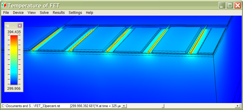
When a solution through time is loaded into the user interface, the software creates a graphical display for each time point in the solution file. For example, a 100µs simulation with solutions written every 10µs would generate eleven different renderings of device temperatures, one for each time point: 0, 10, 20, 30, 40, 50, 60, 70, 80, 90, and 100µs. To examine the solution at these different time points, use the slider at the bottom of the window or the mouse wheel. The time point being displayed is printed to the left of the slider. When only a single time point is present, such as when a steady-state solution is loaded, the slider is disabled.

As shown in the figure below, the temperature scale applies to all time points in the solution. When the temperature scale is configured to display the minimum and maximum temperatures of the data, this range is determined from all the time points in the solution. To get a reading of the device temperatures at a particular time point, scroll the display to that time point and use the temperature range given on the statusbar. Or use the Snapshot... item from the Results menu. A snapshot displays the minimum and maximum temperatures for every component at the current time point, as well as the current settings of the template parameters.

Note: When the display of the solution requires more memory than is available, only part of the solution may be visible. When a solution through time exceeds OpenGL memory, some time points may not be displayed.

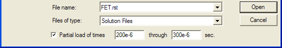
To load only part of a solution through time, use the Load Solution... item from the Solver menu and check the Partial load box at the bottom of the dialog. When the box is checked, the selected solution file will be scanned for the range of time available. Enter a new range to load a subset of the whole file. For example, to load 100µs from the middle of a solution file named FET.rst, use:

Loading a single time point of a solution through time may be useful for examining the solution more closely. The peak temperature values displayed on the temperature scale are determined only from the parts of the solution actually loaded, and the color map displayed will better reflect the temperature range for the time point. Also, a partial solution can be saved in ASCII format for further analysis by using the Save solution as... command from the Solve menu.

Run Values

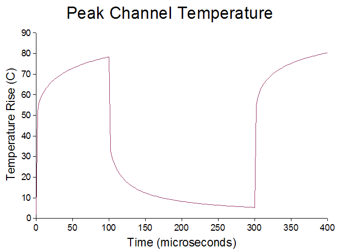
To get a plot of temperature ranges through time, access the recording file (the .csv file) in which specific temperature extremes are written for each time point in the solution. For example, the figure below was produced from the run values recorded for a simulation in which the solution was saved every 2µs. The simulation was performed using the command line utility so that the full solution did not have to be loaded into the graphical user interface to record these results. The plot was generated from OpenOffice Calc.